MxN multi-widget editor: layout as code
The MxN multi-widget editor lets you build arbitrary grids of synchronised render windows. This notebook walks through a multimodal storyline (CT next to MR), and along the way demonstrates the GET-modify-PUT pattern for layout-as-code: the same Python DSL builds layouts from scratch, parses the workbench’s live layout, and validates documents before they cross the network.
You will learn how to:
Open the MxN editor and inspect its current layout
Build a typed
MxNLayoutDocumentand apply it viaset_layoutUse semantic window ids that encode modality and anatomical plane
Drive per-cell node visibility so each cell shows only what it should
Move the crosshair and observe synchronised updates across cells
Prerequisites
A running MITK Workbench at
http://localhost:8080.The MxN multi-widget editor must be open in the workbench before you run the notebook. Open it via Window > New Editor > MxN (or switch to a perspective that includes it).
wb.show()does not open MxN – the StdMultiWidget gets shown instead.The optional
mitkPython package (providesmitk.mxn.layout). This package ships with a local MITK build’s Python wrapping; it is not available from public PyPI. Without it, the typed DSL paths (get_layout,set_layout(doc),update_layout, …) raiseImportError. The raw-dict path (get_layout_json,set_layout(dict)) is always available – see the callout near the end of this notebook.Install the library with the layout extra:
pip install -e ".[layout]"from the repo root.
1. Connect and import the DSL
The DSL is gated on the optional mitk package. We fail loudly with an actionable message if it is missing – the raw-dict path remains usable without it, but every cell below uses the typed builders.
[1]:
import mitk_workbench_remote as mw
from mitk_workbench_remote.examples import phantoms

wb = mw.connect("http://localhost:8080")
if not wb.ping():
    raise SystemExit("Workbench unreachable at http://localhost:8080. Start it and re-run.")

try:
    from mitk.mxn.layout import (
        LayoutWindow,
        MxNLayoutDocument,
        Split,
        ViewDirection,
    )
except ImportError as exc:
    raise SystemExit(
        "This notebook requires the optional 'mitk' package. "
        "Build it from a local MITK CMake build (Wrapping/Python) and install the wheel."
    ) from exc

print(f"Connected to {wb.info.name}; mitk.mxn.layout DSL loaded.")

if not wb.mxn.get_info().active:
    raise SystemExit(
        "The MxN multi-widget editor is not open in the workbench. "
        "Open it via 'Window > New Editor > MxN' and re-run."
    )
Connected to MITK Workbench REST API; mitk.mxn.layout DSL loaded.
2. Two modalities – one body, two textures
We use a deliberately simplified phantom: the body and a small offset tumor. The shape primitives differ by modality so the two volumes are visually distinct – spheres for MR, cubes for CT – but they share the same geometry so they overlay cleanly.
[2]:
mr_image = phantoms.make_body_with_tumor("mr")
ct_image = phantoms.make_body_with_tumor("ct")

mr_node = wb.show(mr_image, name="MR", color=(0.95, 0.30, 0.30))
ct_node = wb.show(ct_image, name="CT", color=(0.30, 0.55, 0.95))
print(f"Loaded {mr_node} and {ct_node}.")
Loaded <DataNode 'MR' (Image) @ /MR uid=node_3> and <DataNode 'CT' (Image) @ /CT uid=node_4>.
3. Open the MxN editor with the default layout
wb.mxn returns a stateless handle to the MxN editor. Out of the box the editor opens with a single cell, so both modalities currently render in the same window. To see them overlaid, we put MR on top and dial its opacity down to 0.5.
[3]:
mxn = wb.mxn
info = mxn.get_info()
print(f"alias={info.alias}  active={info.active}  cells={info.windows}")

# Stack MR above CT and make MR semi-transparent so both modalities are visible.
for cell in mxn.list_windows():
    cell.set_node_layer(ct_node, 0)
    cell.set_node_layer(mr_node, 1)
mr_node.opacity = 0.5
wb.update()
print("MR is on top at 50% opacity.")
alias=mxn  active=True  cells=('mxn__ct_axial', 'mxn__ct_coronal', 'mxn__ct_sagittal', 'mxn__mr_axial', 'mxn__mr_coronal', 'mxn__mr_sagittal')
MR is on top at 50% opacity.
Try this: open the workbench’s data inspector for the active cell. Both MR and CT are listed – in this default single-cell layout, every visible node renders in every window.
4. Layout as code: GET the current document
mxn.get_layout() parses the live workbench layout into a typed MxNLayoutDocument. Repr is human-readable; to_json() shows the wire form.
[4]:
current = mxn.get_layout()
print(current)
MxNLayoutDocument(name='modality grid', version='2.0', windows=6, groups=2)
Layouts also support pretty html print/representation.
[5]:
current
[5]:
| |||
|
Build a one-row, three-plane layout
A common quick-look layout is a single row of three cells, one per anatomical plane, all linked to the same selection group. We construct the windows manually so the cell ids encode the plane (mxn__row_axial etc.) – semantic ids make the next steps easier to read.
[6]:
row_doc = MxNLayoutDocument.create(
    root=Split.horizontal(
        LayoutWindow.create(
            id="mxn__row_axial",
            view_direction=ViewDirection.AXIAL,
            selection="main",
            name="Axial",
        ),
        LayoutWindow.create(
            id="mxn__row_coronal",
            view_direction=ViewDirection.CORONAL,
            selection="main",
            name="Coronal",
        ),
        LayoutWindow.create(
            id="mxn__row_sagittal",
            view_direction=ViewDirection.SAGITTAL,
            selection="main",
            name="Sagittal",
        ),
    ),
    name="multimodal row",
)
mxn.set_layout(row_doc)
print(f"Cells now: {[c.id for c in mxn.list_windows()]}")
row_doc
Cells now: ['mxn__row_axial', 'mxn__row_coronal', 'mxn__row_sagittal']
[6]:
Axial mxn__row_axial view: axial selection: main | Coronal mxn__row_coronal view: coronal selection: main | Sagittal mxn__row_sagittal view: sagittal selection: main |
Try this: look at the workbench. Three cells, one per plane, all showing both modalities. Because every cell is in the same main selection group, selecting a node in one cell selects it in the others. MR is still at 50% opacity from step 3 – both modalities are visible as a coregistered overlay in every cell.
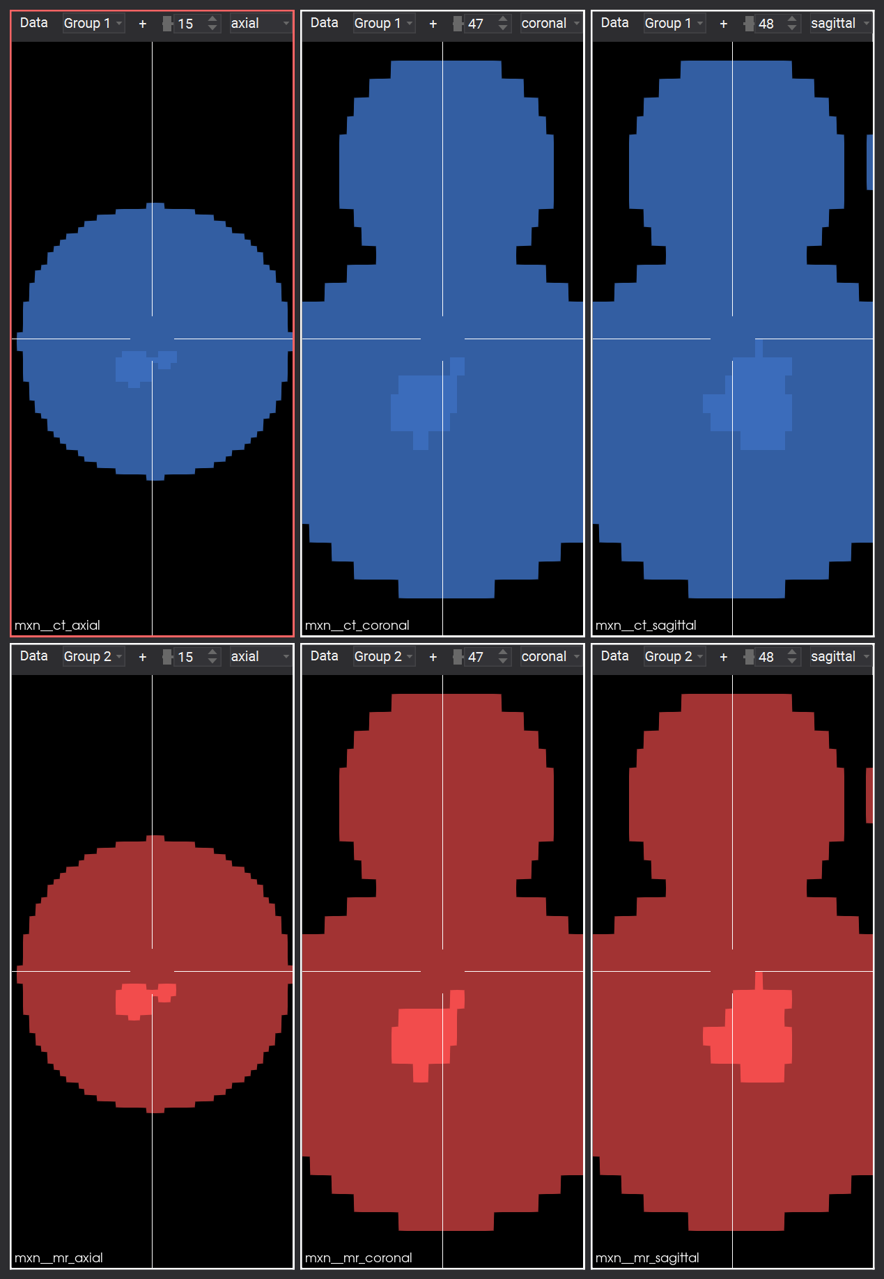
5. A 2x3 modality grid with per-row groups
To put each modality in its own row we build a 2x3 grid. Two synchronisation groups (ct and mr) keep the rows independent – selection state in the CT row does not leak into MR. Window ids encode both modality and plane (e.g. mxn__ct_axial).
[7]:
def make_row(modality: str) -> Split:
    label = modality.upper()
    return Split.horizontal(
        LayoutWindow.create(
            id=f"mxn__{modality}_axial",
            view_direction=ViewDirection.AXIAL,
            selection=modality,
            name=f"{label} axial",
        ),
        LayoutWindow.create(
            id=f"mxn__{modality}_coronal",
            view_direction=ViewDirection.CORONAL,
            selection=modality,
            name=f"{label} coronal",
        ),
        LayoutWindow.create(
            id=f"mxn__{modality}_sagittal",
            view_direction=ViewDirection.SAGITTAL,
            selection=modality,
            name=f"{label} sagittal",
        ),
    )

# Keep the rows as named locals: the per-cell visibility step in the
# next cell iterates them directly, so it never has to recover the
# row-to-cell mapping by pattern-matching cell ids.
ct_row = make_row("ct")
mr_row = make_row("mr")

modality_doc = MxNLayoutDocument.create(
    root=Split.vertical(ct_row, mr_row),
    name="modality grid",
)
mxn.set_layout(modality_doc)
print(f"Cells now: {[c.id for c in mxn.list_windows()]}")
print(f"Groups:    {sorted(modality_doc.groups)}")
modality_doc
Cells now: ['mxn__ct_axial', 'mxn__ct_coronal', 'mxn__ct_sagittal', 'mxn__mr_axial', 'mxn__mr_coronal', 'mxn__mr_sagittal']
Groups:    ['ct', 'mr']
[7]:
| |||
|
Per-cell node visibility
The layout determines which cells exist; node visibility per cell is a DataNode property scoped by the cell’s render context. The library wraps this as RenderWindow.set_node_visible(node, True/False) – the cell id is threaded through as the property’s context query parameter.
[8]:
# Iterate the cached row Splits from the previous cell rather than
# recovering the mapping from cell-id prefixes. The DSL nodes you used
# to build the layout are also the cleanest iteration source.
for win in ct_row.windows():
    cell = mxn[win.id]
    cell.set_node_visible(ct_node, True)
    cell.set_node_visible(mr_node, False)

for win in mr_row.windows():
    cell = mxn[win.id]
    cell.set_node_visible(ct_node, False)
    cell.set_node_visible(mr_node, True)

# With each modality confined to its own row, the 50% MR overlay is no
# longer needed.
mr_node.opacity = 1.0
wb.update()
print("Per-cell visibility set; MR opacity restored to 1.0.")
Per-cell visibility set; MR opacity restored to 1.0.
Try this: the data inspector now shows only the relevant modality per cell. CT lives in the top row, MR in the bottom row, and the per-row selection groups keep navigation independent within each modality.
6. Snapshot the editor
mxn.screenshot() grabs the entire MxN canvas (cell tree only – no toolbars or side panels). It returns raw PNG bytes; we render inline via matplotlib.
[9]:
from IPython.display import Image as IPyImage

IPyImage(data=mxn.screenshot(), format="png", width=300)
[9]:
JSON-only path (no mitk install)
The same flow runs without the optional DSL by trading typed builders for raw dicts:
mxn.get_layout_json()returns the JSON body unchanged.mxn.set_layout(payload)accepts adictand PUTs it as-is. The server validates the schema and returns 400INVALID_REQUESTon a malformed body.
The dict shape mirrors the schema (mxn-layout-v2.schema.json) one-to-one and is byte-stable with what get_layout_json returns. Use this path in environments where a local MITK build is not available; lose only the client-side validation and the ergonomic builders.
Recap and clean up
What you exercised:
MxNEditor.get_info,get_layout,set_layout,screenshotMxNRenderWindow.set_node_visible,set_node_layerWorkbench.set_positionDSL building blocks:
LayoutWindow,Split,MxNLayoutDocument, selection-linked groups viaselection="<name>"Semantic, plane-encoding cell ids that route end-to-end (URL, document, engine) without prefix translation
Notebook 08 reuses these primitives in a cohort-processing script.
[10]:
mr_node.remove()
ct_node.remove()
print("Removed CT and MR nodes.")
Removed CT and MR nodes.