show() and basic Rendering Control
This notebook demonstrates the wb.show() convenience method – the primary one-liner for getting data into the Workbench – and the fundamental rendering control endpoints (position, screenshot).
You will learn how to:
Show data with a single call:
wb.show(array, name=..., color=..., opacity=...)Show a file from disk without loading it into Python
Control parent nodes, visibility, and reinit behavior
Use the fine-grained alternative (
storage.create()+node.set_data()+node.update_properties())Read and set the crosshair position
Capture screenshots and display them inline
Hint: In the rest of the notebook explanation “mw” is referring to the mitk_workbench_remote package.
Prerequisites: A running MITK Workbench instance with the REST API enabled.
1. Connect to a running Workbench
[1]:
import numpy as np
import mitk_workbench_remote as mw

instances = mw.discover(timeout=2)
if not instances:
    raise SystemExit("No running MITK Workbench found. Start one and try again.")

wb = instances[0]
print(f"Connected to: {wb.info.name} (MITK {wb.info.mitk_version}) at {wb.url}")
Connected to: MITK Workbench REST API (MITK 2025.12.99-2c35144d) at http://localhost:8080
2. show() basics
wb.show() is the primary one-liner for displaying data in the Workbench. It combines node creation, data upload, property setting, and reinit into a single call.
It accepts mw.Image objects, mw.MultiLabelSegmentation objects, any types that can be converted into mw.Image (e.g. numpy arrays, SimpleITK images, MLArray objects) or file paths. The return value is the newly created DataNode.
[2]:
# Create a synthetic 3D gradient volume
size = 64
arr = np.sum(np.indices((size, size, size), dtype=np.float32), axis=0)
arr /= arr.max()

# Show it in the Workbench with a custom name, color, and opacity
node_gradient = wb.show(arr, name="Gradient", color=(0.2, 0.6, 1.0), opacity=0.8)
print(f"Created node: {node_gradient}")
Created node: <DataNode 'Gradient' (Image) @ /Gradient uid=node_1>
You can also pass an mw.Image with full spatial metadata (spacing, origin, direction):
[3]:
# Create a sphere phantom with custom spacing
sphere = np.zeros((64, 64, 64), dtype=np.float32)
center = np.array([32, 32, 32])
for idx in np.ndindex(sphere.shape):
    dist = np.linalg.norm(np.array(idx) - center)
    sphere[idx] = max(0, 1.0 - dist / 20.0)

image = mw.Image(sphere, spacing=(0.5, 0.5, 0.5), origin=(16.0, 16.0, 16.0))
node_sphere = wb.show(image, name="Sphere", color=(1.0, 0.3, 0.0))
print(f"Created node: {node_sphere}")
Created node: <DataNode 'Sphere' (Image) @ /Sphere uid=node_2>
3. show() with a file path
When you pass a file path (string or Path), show() uploads the raw bytes directly without deserializing the file into Python. The Workbench server parses the file format. This is the most efficient way to load existing files. As long as the MITK Workbench knows this format it will be automatically handled.
The node name is inferred from the file stem (e.g. "ct_scan.nrrd" becomes "ct_scan").
[4]:
from pathlib import Path

# Save the sphere to a temporary NRRD file and re-show it from disk
tmp_file = Path("sphere_example.nrrd")
node_sphere.save_data(tmp_file)

node_from_file = wb.show(tmp_file, name="FromFile", color=(0.0, 1.0, 0.5))
print(f"Loaded from file: {node_from_file}")

# Clean up the temp file
tmp_file.unlink(missing_ok=True)
''
Loaded from file: <DataNode 'FromFile' (Image) @ /FromFile uid=node_3>
[4]:
''
4. show() as a child node
Use the parent parameter to create the new node as a child of an existing node. This is useful for organizing related data (e.g. a segmentation under its source image).
[5]:
#remove the FromFile node to avoid cluttering the view
node_from_file.remove()

# Create a binary mask and show it as a child of the sphere node
mask = (sphere > 0.5).astype(np.uint8)
node_mask = wb.show(mask, name="ThresholdMask", parent=node_sphere, color=(1.0, 1.0, 0.0))
print(f"Child node: {node_mask}")
print(f"Parent path: {node_sphere.path}")
print(f"Child path:  {node_mask.path}")
Child node: <DataNode 'ThresholdMask' (Image) @ /Sphere/ThresholdMask uid=node_4>
Parent path: /Sphere
Child path:  /Sphere/ThresholdMask
5. hide_others
When hide_others=True, all existing nodes are hidden before the new data is shown. This is handy when you want a clean view of just the new data.
[6]:
# Show a new volume while hiding everything else
solo = np.random.default_rng(42).random((32, 32, 32), dtype=np.float32)
node_solo = wb.show(solo, name="SoloView", hide_others=True, color=(0.8, 0.2, 0.8))
print(f"Only '{node_solo.name}' is visible now.")
Only 'SoloView' is visible now.
6. ReinitMode
By default show() calls a global reinit (ReinitMode.ALL_VISIBLE) to fit all views to all visible data. You can change this behavior:
ReinitMode.ALL_VISIBLE(default) – global reinit: fits views to all visible dataReinitMode.NODE– fits views to just the newly shown nodeReinitMode.NONE– skips reinit entirely (useful e.g if you want to add something w/o altering the scene)
[7]:
# Load a volume without reinit, then reinit once at the end
small_1 = np.random.default_rng(1).random((16, 16, 16), dtype=np.float32)

n1 = wb.show(small_1, name="Batch1", reinit=mw.ReinitMode.NONE)

# Now reinit to fit everything
print(f"Loaded {n1.name} w/o reinit.")
Loaded Batch1 w/o reinit.
[8]:
# ReinitMode.NODE -- fit views to just the new node
big = np.zeros((128, 128, 128), dtype=np.float32)
big[40:90, 40:90, 40:90] = 1.0
node_big = wb.show(big, name="BigCube", reinit=mw.ReinitMode.NODE)
print(f"Views now fit to '{node_big.name}' only.")
Views now fit to 'BigCube' only.
7. Fine-grained alternative
wb.show() is a convenience wrapper. Under the hood it calls:
wb.storage.create(name, parent=...)– create an empty nodenode.set_data(data)– upload datanode.update_properties(visible=..., opacity=..., color=..., context=...)– set display properties (usecontext=for per-render-window properties)wb.reinit()orwb.reinit([node])– reinit the views
You can call these steps individually for more control.
[9]:
# Equivalent of: wb.show(arr, name="Manual", color=(0.0, 1.0, 0.0), opacity=0.6)
manual_node = wb.storage.create("Manual")
manual_node.set_data(mw.Image(arr))
manual_node.update_properties(visible=True, opacity=0.6, color=(0.0, 1.0, 0.0))
wb.reinit([manual_node])
print(f"Created manually: {manual_node}")
Created manually: <DataNode 'Manual' (Image) @ /Manual uid=node_12>
8. Position control
The crosshair position can be read and set in world coordinates. get_position() also returns the scene bounding box (the axis-aligned bounding box of all loaded geometry), which is useful for navigating to specific locations.
[10]:
# Read the current crosshair position and scene bounds
pos = wb.get_position()
print(f"Crosshair: {pos.position}")
print(f"Bounds min: {pos.bounds.min_position}")
print(f"Bounds max: {pos.bounds.max_position}")
Crosshair: (32.0, 31.0, 31.0)
Bounds min: (-0.5, -0.5, -0.5)
Bounds max: (63.5, 63.5, 63.5)
[11]:
# Navigate to the center of the scene bounding box
if pos.bounds.min_position is not None and pos.bounds.max_position is not None:
    center = tuple(
        (lo + hi) / 2.0
        for lo, hi in zip(pos.bounds.min_position, pos.bounds.max_position)
    )
    wb.set_position(center)
    print(f"Moved crosshair to center: {center}")
else:
    print("No geometry loaded -- bounds are None.")
Moved crosshair to center: (31.5, 31.5, 31.5)
9. Screenshot
Capture a screenshot of the active Workbench window. The image is returned as raw bytes (PNG or JPEG). You can optionally scale the output and save to a file.
In Jupyter, use IPython.display.Image to display the screenshot inline.
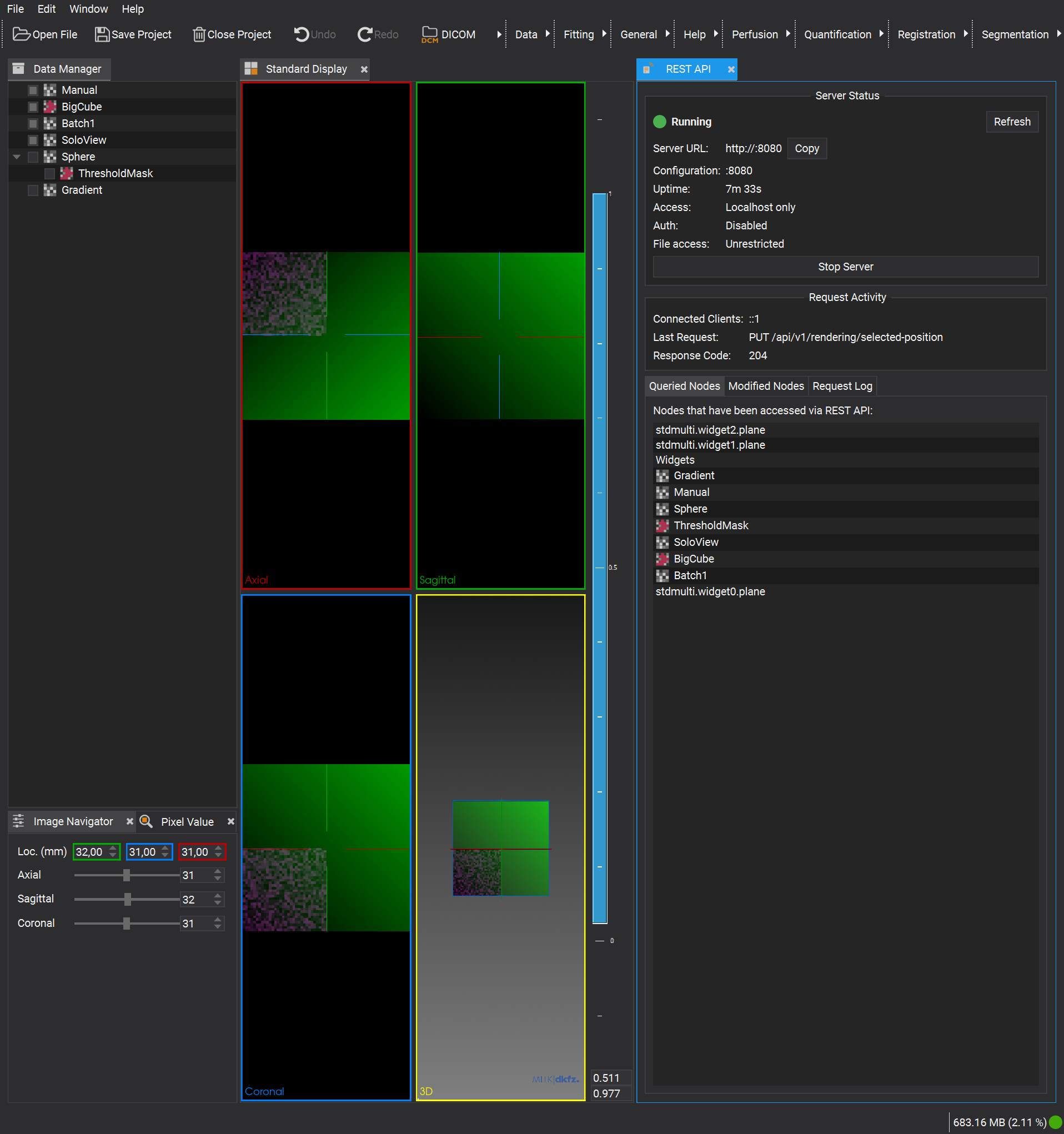
[12]:
from IPython.display import Image as IPImage, display

# Capture at default resolution
png_bytes = wb.screenshot()
print(f"Screenshot: {len(png_bytes)} bytes")
display(IPImage(data=png_bytes))
Screenshot: 266972 bytes
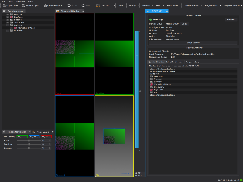
[13]:
# Capture with specific dimensions
scaled = wb.screenshot(width=800, height=600)
print(f"Scaled screenshot: {len(scaled)} bytes")
display(IPImage(data=scaled))
Scaled screenshot: 99027 bytes
[14]:
# Save screenshot to file
wb.screenshot(path="workbench_capture.png")
print(f"Saved to workbench_capture.png ({Path('workbench_capture.png').stat().st_size} bytes)")

# Clean up
Path("workbench_capture.png").unlink(missing_ok=True)
Saved to workbench_capture.png (266605 bytes)
10. Clean up
Remove all nodes we created in this notebook.
[15]:
for node in [node_gradient, node_sphere, node_solo,
             n1, node_mask, node_big, manual_node]:
    try:
        node.remove(recursive=True)
    except Exception:
        pass  # node may already be gone (e.g. child removed with parent)

print("Done.")
Done.